
Nyquist Signal Expansion with Python
I’ve recently been reading up on software defined radio (SDR). An epiphany that I had recently was that if we have sampled a signal so that we meet the Nyquist criteria, we can reproduce the points between the points we took.You may have clued in on this previously, but it only just clicked for me. Most of this post is brought to you by the letters ‘S’, ‘D’, ‘R’ and Signal Processing Techniques for Software Radios, Second Edition by Behrous Fahang-Boroujeny. Example 5.1 in his book is the basis for much of what is shown here.
[notice]This post gets kind of theoretical. Consider yourself warned.[/notice]
Now, why do you care? Let’s say that we have successfully sampled our signal at a speed that satisfies the Nyquest criterion, $latex t_s \le \frac{1}{2f_{max}}$ where ts is the time between samples and fmax is the maximum frequency in the signal. What if we didn’t sample it quite when we wanted to, relative to the signal. The sampling rate is the same, but we have an offset, Δt. By digitally resampling the signal we can remove Δt from the signal. We can even find what Δt is without human intervention. I had to prove it to myself first. After proving it to myself I’ve got several fields I want to apply this to besides SDR. That’s why you should care. Now, for the explanation.
Following Along
If you would like to follow along, you just need a computer with python and the numpy, scipy, and matplotlib modules. Two easy ways to get this for windows are the python(x,y) distribution or the Enthought python distribution. If you are running Linux, you should be able to install the modules using your preferred packaging system.
If you are also following along from Example 5.1 in Signal Processing Techniques for Software Radios, Second Edition, please remember that MATLAB is a one (1) based indexing language, not zero (0) based like a proper programming language. Python is zero (based). Forgetting this will result in banging your head against the keyboard in frustration. I know.
Generating the Initial Signal and Samples
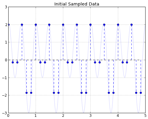
To generate the initial signal and its sample points (see Figure 1), we use the following code:
import scipy.signals as signals
import matplotlib.pyplot as plt
fs_in = 6
#remember python does integer division if the divisor is an integer
Ts_in = 1/float(fs_in)
t_in = np.r_[0:5:Ts_in]
x_in = np.sin(2*np.pi*t_in) + 2*np.cos(4*np.pi*t_in)
t_cont = np.r_[0:5:0.01]
x_cont = np.sin(2*np.pi*t_cont) + 2*np.cos(4*np.pi*t_cont)

Figure 1. Initial signal generated for this example. Dots are the samples taken.
Expanding
Now that we have the original signal, we need to expand it. To expand it we place N samples between each original sample. These new samples are all zero (0). Below is a python function to mimic the expander() function in MATLAB:
xout = np.zeros(x_in.size*L)
xout[::L] = x_in
return xout
For this example we will expand by L = 3. Our sampled data now looks like:

Figure 2. What our data looks like now that we have expanded it by L=3
The next step is where the magic happens.